Understanding Big O Notation: A Beginner's Guide

Why should I learn about Big O Notation?
Because it is commonly asked in tech interviews, one can say.
The reason that many tech companies test their candidate's knowledge of big O notation is to check if the candidate can write efficient code and is aware of what kinds of code are expensive to run, both in terms of actual money and resources, such as computer memory or processing time.
It is important to write code that runs without errors and outputs the expected result, but there is a third component in it, which is efficiency.
A company that hosts its services on cloud servers, such as AWS or Google Cloud, can save millions just by replacing an inefficient code with an efficient one. With optimization, it is possible to do the same work on a much cheaper server or spend less computing time. This is just an example where just by changing a piece of code it is possible to save millions of dollars, so no wonder it is essential for companies to search for programmers that can write efficient code.
Even if you are writing just simple scripts, a skill that empowers you to look at a piece of code and lets you know which parts of it are critical to performance will empower you to always make the best decisions to build a fast program that can serve millions of users or process huge loads of data in no time.

So let's learn about big O notation!
What is Big O Notation?
Big O notation is always pessimistic. Suppose I have a list that contains thousands of names:
# I have a long list of names
names = ['Ed', 'Karl', 'Sam', 'Ana', thousands of names, 'Boris']
Imagine that I have a program that searches for a name in the names list. One way for a computer to search a list is by checking one item at a time. If the name to be found is "Sam", as humans we can just look at the above list and find it, but with computers, the process goes like this:
First item at index 0 is Ed. Is Ed equal to Sam? No
Second item at index 1 is Karl. Is Karl equal to Sam? No
Third item at index 2 is Sam. Is Sam equal to Sam? Yes
Sam was found at index 2
The same process happens in the following Python code:
# For each name in names list
for name in names:
  # If name is equal to 'Sam'
  if name == 'Sam':
    # Returns True
    return True
# If 'Sam' was not found in the list, return False
return False
The best-case scenario is finding "Ed". Ed is the first item on the list, so it will be found very fast, regardless of the list size. But as programmers, we always need to think in terms of the worst-case scenario, because they are the ones responsible for problems.

The worst-case scenario is a name that is not on the list. A computer will have to check all names in this huge list, one by one, only to tell us that the name is not on the list.
Big O notation is interested only in the worst-case scenario. In simple terms, it gives a grade to the performance of a task in the worst-case possible.
The process I described here to find a name on a list can be defined as an algorithm. Do not let its fancy name deceive you.

An algorithm is just a list of steps that are needed to solve a problem. You can think of these real-world examples that are equivalent to an algorithm:
Directions from home to a bakery: From your home, turn right, walk 500 meters, turn left, cross a bridge, and walk 50 meters. You will reach the bakery.
A recipe for fried egg: Take a frying pan and put one tablespoon of oil on it. Place it on medium heat. Break one egg in the frying pan. Cook until the egg yolk becomes solid. You have a fried egg!
From now on, instead of saying a task, a program or code, I will use "algorithm".
When does efficiency matter?
If my algorithm is dealing with a small input, like a list with 10 items, it will not benefit from optimization, as any algorithm will complete the task in some milliseconds, with no notable difference between the top and worst performers. An algorithm that orders a list of numbers with only 10 items will not benefit much from optimization, as it will be done in a very short time, regardless of its performance.
Most users would be satisfied with a process that takes less than a second to complete, but as the size of the list increases, performance can suffer to a point that even a human can feel.
Below you can find a comparison between an okay algorithm and a bad one. It shows how many operations are needed as we increase the size of a list.
You will see later what O(n) and O(n2) mean.
| Number of operations | Number of operations | |
| Size of the list | Ok algorithm: O(n) | Bad algorithm: O(n2) |
| 2 | 2 | 4 |
| 10 | 10 | 100 |
| 1.000 | 1.000 | 1.000.000 |
| 10.000 | 10.000 | 10.0000.000 |
When the size of the list is small, the number of operations in the worst case remains small. But when the size begins to increase from 1.000 onwards, the discrepancies between an okay algorithm and a bad algorithm become very evident.
Some algorithms can take months or thousands of years to complete a task if an inefficient algorithm is used because they have to deal with huge amounts of data, think about big data or machine learning. Or it will not have practical applicability if a result cannot be found in a very short time, think about calculating a route in Google Maps or giving product recommendations at Amazon. Google would not have a viable product if returning a route from point A to point B would take 15 minutes.
The types of efficiency, from best to worst
Constant Time: The Gold Standard
Representation: O(1)
This is the most efficient algorithm. An algorithm that has a constant time takes the same amount of time to get the task done, regardless of the size of the input. By input, here I mean the length of the list. Normally as the length increases, the time required to do a certain task increases, but not when we are dealing with a constant time algorithm.
I will list some operations that are done in constant time:
names[-1] # Gets the last item of a list
# Returns Boris

names[-1] = 'Clara' # Sets the last item as Clara

names.append('Marcus') # Appends 'Marcus' to the end of the list

names.pop() # Removes the last item from the list
All these operations take the same time, regardless if a list has one name or thousands of names. Also, there is no difference between best-case and worst-case here.
This may look strange because I have said previously that a computer must look for all items on a list when searching for a value. But when the index of the item is known or we know that we are dealing with the last item, there is no need to hop from item to item. When using append() or pop() we don't have to go through the items on the list because we only want to change the end of the list and we know where the last item is located.
If we create a graph with the time needed for the algorithm to complete versus the volume of data, the result will be this:
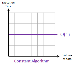
The time remains the same, regardless of the input size. The number of operations of O(1) is 1, meaning only a single operation is needed to finsih the algorithm.
Logarithmic: Divide and conquer
Representation: O(log n), where n is the size of the list
Remember that we were searching for a name on a list? If the list was sorted alphabetically, it would be possible to search more efficiently. Suppose I am searching for the name "Hagar", which begins with "H":
# We have sorted the list alphabetically
sorted_names = ['Ana', 'Boris', 'Ed', 'Karl', 'Sam', thousands of sorted names, 'Zara']
# size of the list: 10.000

# Get to the middle of the list, divide the list in two
# Is the letter H in the left list or in the right list?
divided_names = ['Ana', ..., 'Marcus'] + ['May', ..., 'Zara']
# size of left list: 5.000
# size of right list: 5.000

# As H is between A and M, we can safely discard the right list, reducing the problem in half!
sorted_names = ['Ana', ..., 'Marcus']
# size of the list: 5.000

# We again get the middle of the list and divide it in two, repeating the process
divided_names = ['Ana', ..., 'Fred'] + ['Frodo', ..., 'Marcus']
# size of left list: 2.500
# size of right list: 2.500

# H should be on the right list, we again reduced the problem in half!
sorted_names = ['Frodo', ..., 'Marcus']
# size of the list: 2.500

# Continues until there is one name left in the list
The worst-case situation would be not finding a name on the list.
As you can see, by dividing the list size by half, we are also dividing the size of the problem by half. This is much more efficient than checking all the items one by one.
This makes sense if we think of real-life examples. The contacts list on our phones is organized by name and as a result, we can quickly find the contact name we want. Searching for a contact in the contacts list is a very common task, so the programmers of the phone book app already sorted the contact list alphabetically for us. It would be much harder to find a contact if the contacts were sorted by the date they were added or if they were shown in a random order.
If we apply this principle to code, if we know that a list will be searched many times, we can optimize the time needed to do these searches by sorting the list beforehand. Sorting is a costly process in terms of time, but this cost is only paid once, so it is worthwhile in cases where we know that we are going to do multiple searches.
The graph of a logarithmic algorithm will be:

It starts to increase, but as the input size gets larger, the execution time begins to flatten. It gets more efficient as the input size gets larger.
O(log n) means that the number of operations needed in the worst case is log n. For example, log(4) is 2, which is just half, but log(100) is 6.644 and log(1000) is 9.966. You can see that the number of operations remains small even with a list with a huge size.
Linear: The predictable algorithm
Representation O(n), where n is the size of the list
The process I described when trying the find a name on a list is classified as a linear algorithm. It checks for every item on a list in its worst case, so the time needed to do this depends on the size of the list.
The code below is equivalent to the example I refer to above:
# For each name in names list
for name in names:
  # If name is equal to 'Sam'
  if name == 'Sam':
    # Returns True
    return True
# If 'Sam' was not found in the list, return False
return False
Sometimes a single line of code has the same complexity as the code above:
if 'Sam' in names:
    return True
return False
The part 'Sam' in names has a time complexity of O(n), despite being a single line. The underlining process is the same: it still has to go through all items in the list if the name is not on the list.
When analyzing a piece of code, always think about the principles of how a computer completes the task. To look for the name Sam in the names list, it still has to search one name at a time, despite being a one-liner and inside an if condition.
The graph below shows what a linear algorithm looks like:
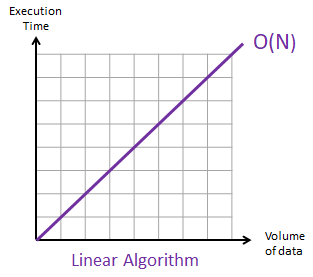
As the size of the list increases, the time needed follows together.
Danger Zone: Things could start to get slow from here
Quadratic:
Representation: O(n²)
Imagine that I want to check if there is a duplicate name in the list of names.
# I have a long list of names
names = ['Ed', 'Karl', 'Sam', 'Ana', thousands of names, 'Boris']

# For each name in names list
for index1, name1 in enumerate(names):
  # Loop through the list again
  for index2, name2 in enumerate(names):
    # Only make a comparison when indexes are different
    if index1 != index2:
      # If names are equal, print message with the duplicate name
      if name1 == name2:
        print(f'A duplicate name was found: {name1}')
Here enumerate() allows me to keep track of indexes of the list without needing to use range() and len() allowing me to write a simpler and cleaner code.
This algorithm starts almost the same as a linear algorithm, with a for loop, but it has an important difference. There is another for loop inside the first loop! It means that: For each name in the list, we have to loop through all names in the list!
The worst-case scenario would be any run because this time the algorithm continues to run until the end of the list even if a duplicate was found. Even I can feel the amount of work that the poor computer would need to perform!
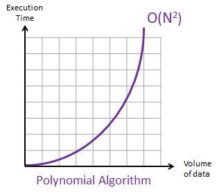
The graph looks like an inverted logarithmic graph: As the input size gets larger, the execution time increases drastically.
Exponential
Representation O(2ˆn)
I have a list with a single name and I want to generate all the possible combinations. There would be two possible combinations:
One with the name "Ed"
One empty list, without the name "Ed"
name = ['Ed']

ed_present = ['Ed']
ed_absent = []

# Let's combine all possibilities

scenario1 = ['Ed']
scenario2 = []
Now, what if I wanted all combinations from a list with two names?
The process would be the same, for each name, the name can be included or excluded:
names = ['Ed', 'John']

# Ed can be present or absent
ed_present = ['Ed']
ed_absent = []

# John can be present or absent
john_present = ['John']
john_absent = []

# Let's combine all possibilities
scenario1 = ['Ed', 'John'] #combining ed_present + john_present
scenario2 = ['Ed'] #combining ed_present + john_absent
scenario3 = ['John'] #combining ed_absent + john_present
scenario4 = [] #combining ed_absent + john_absent
We can see a pattern here, we can multiply the resulting 2 possibilities of Ed with the 2 possibilities of John so we get 4.
names = ['Ed', 'John', 'Maria']

# Ed can be present or absent
ed_present = ['Ed']
ed_absent = []

# John can be present or absent
john_present = ['John']
john_absent = []

# Maria can be present or absent
maria_present = ['Maria']
maria_absent = []
With 3 elements, the total combinations would be 2 x 2 x 2, which would result in 8.
To calculate the necessary steps to go through all combinations, we can calculate 2 to the power of the length of the list, or 2 ˆ <list_length>, as we saw in the previous examples:
With a list of length 1: 2 ^ 1 = 2
With a list of length 2: 2 ^ 2 = 4
With a list of length 3: 2 ^ 3 = 8
This can get ugly very fast, as with a length of 20 you will be returning 1,048,576 combinations and with a length of 63, it will return a whooping 9,223,372,036,854,775,808 combinations.
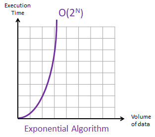
As you can see, the rate of growth of an algorithm with exponential complexity is very steep and it is very slow.
Conclusions
Although some algorithms are better than others, some problems are not possible to be solved with a good algorithm and we need to stick with a bad algorithm, as it is our only option. If we need to search for an item on a list, there is no way we can achieve this in a constant time or O(1).
As we saw, there are creative ways to increase efficiency, by transforming a linear algorithm O(n) to a logarithmic O(log n) by sorting the list before searching and then dividing the problem in half. In this case, it will be worth it if you plan to do multiple searches on the list, as there is a cost for sorting the list.
In this article, I gave examples related only to lists, but any input is applicable here. It could be integers, dictionaries, and so on, but I chose lists because most of my readers would be more comfortable with them.
When trying to determine the complexity of an algorithm you wrote, keep the big picture. Keep an eye out for loops as they are the main cause of increases in complexity. However spotting a loop can be a challenge, as it can be disguised as something else:
# This line below appears to be simple, but has a complexity of O(n)
if 'Kenya' in names:
  print('Found Kenya')
In the example above, it appears that this is only an if cause, which can be safely ignored, but if you think about it, it needs to iterate a list to find the name "Kenya". It does the same as :
# This loop has a complexity of O(n)
for name in names:
  if name == 'Kenya':
    print('Found Kenya')
Final Considerations
When writing an algorithm for the first time, you should not aim for performance. Instead, aim for an algorithm that does the job correctly. Then, if the need arises, you should start optimizing it to go faster. Remember: Premature optimization is the root of all evil
Hope you liked this article! If you have questions or comments, please write them in the comments section :)